A reverse tax formula in Google Sheets removes included tax by dividing the gross amount by the tax multiplier in a spreadsheet cell. The net formula returns the before-tax price, while a second formula subtracts net from gross to show the tax already included. Google Sheets calculations need clean rate cells, decimal formatting, copied formulas, and separate rows for mixed rates, exempt items, discounts, shipping, and rounded receipt totals.
This page explains how to set up the formula in Google Sheets, how to avoid rate-format mistakes, how to build QA checks, and how to handle multiple rows, shown tax amounts, VAT, GST, and mixed receipts.
What Is the Google Sheets Reverse Tax Formula?
If the tax-inclusive total is in A2 and the tax rate is in B2, use:
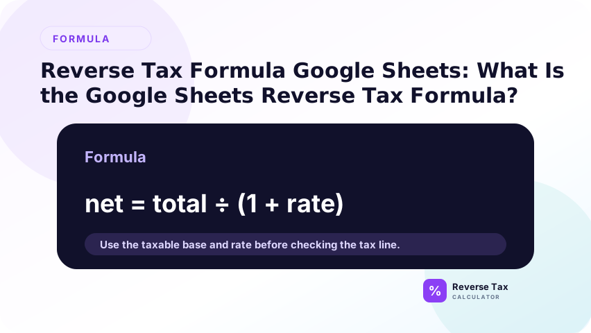
=A2/(1+B2)
If A2 is $108.00 and B2 is 8%, Google Sheets returns $100.00. The formula assumes the total already includes tax and the rate is entered as a percentage or decimal.
This formula should be used only after the row is confirmed as tax-inclusive. If A2 is a subtotal before tax, the formula will incorrectly reduce it. Add a price-type column when the sheet contains mixed source data.
How Do You Calculate Tax Amount?
Use:
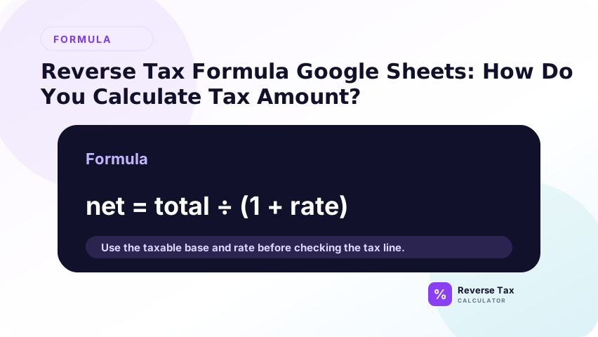
=A2-(A2/(1+B2))
This subtracts the calculated before-tax amount from the tax-inclusive total. Keeping this in a separate column makes the sheet easier to audit and easier to troubleshoot when the receipt does not match.
The tax amount column should not overwrite a shown tax amount from the receipt. If the source already provides tax, keep it in a separate column and use the calculated amount only for checking or variance analysis.
How Should the Rate Be Entered?
Enter the rate as 8% or 0.08. If users enter whole numbers like 8, create a normalized rate column:

=B2/100
Then reference the normalized rate in the formula. This avoids one of the most common spreadsheet errors in tax calculations.
Rate formatting should be tested before formulas are copied down. Entering 8 instead of 8% can make the divisor 9 instead of 1.08, which creates a wildly wrong before-tax amount. Normalization makes the expected rate format explicit.
Google Sheets Example Table
| Total including tax | Rate | Before-tax amount | Tax amount |
|---|---|---|---|
| $108.00 | 8% | $100.00 | $8.00 |
| $113.00 | 13% | $100.00 | $13.00 |
| $120.00 | 20% | $100.00 | $20.00 |
The formula changes only because the rate changes. The structure stays the same.
Why You Should Not Use One Minus Rate
Do not use =A2*(1-B2) for reverse tax. That subtracts the tax percentage from the total and produces the wrong before-tax amount.
At 8%, $108.00 times 0.92 equals $99.36, but the correct before-tax amount is $100.00. The issue is explained more deeply in the subtracting tax percentage guide.
This mistake is common because it resembles a discount formula. Reverse tax is not a discount. It must undo the original tax multiplier, so the formula needs division by 1+rate, not multiplication by 1-rate.
How to Build a Rebuilt Total Check
Add a rebuilt total column:
=BeforeTaxAmount+TaxAmount
Then add a variance column:
=OriginalTotal-RebuiltTotal
The variance column catches wrong rates, source totals, rounding differences, and mixed rows. A variance above one cent should be reviewed.
This check is the most important QA feature in the sheet. It confirms whether the calculated before-tax amount and tax amount return to the original source total. If they do not, the row needs review before it is used.
How to Use ARRAYFORMULA Safely
Google Sheets users often want formulas that fill automatically. An ARRAYFORMULA can work, but it should not calculate rows where price type or rate is blank.
Use helper columns and conditions rather than one huge formula. A clear sheet is easier to audit than a clever formula that hides several decisions.
For example, an array formula should skip rows where tax rate or total is blank. It should also avoid calculating rows marked as shown-tax or mixed unless the logic explicitly handles those cases. Automatic fill is useful only when classification is reliable.
How to Handle Multiple Rows
For multiple rows, use a price type column before applying formulas. Mark rows as tax-inclusive, tax-exclusive, shown-tax, or mixed.
The multiple spreadsheet rows workflow explains why row classification should happen before formula fill. This is especially important in shared sheets.
Shared sheets often collect rows from different users or systems. One row may be a receipt, another may be an invoice, and another may be a payout. Classification keeps one formula from being applied to different evidence types.
How to Handle Shown Tax Amounts
If the receipt shows the tax amount, use:
=Total-ShownTaxAmount
This respects the source document's rounding. Use the rate-based formula only when tax amount is missing or when you are checking the shown value.
Shown tax should usually be treated as source evidence. A calculated tax amount may differ by a cent because of rounding, so replacing shown tax with calculated tax can create unnecessary mismatch problems.
How to Handle VAT and GST
VAT and GST use the same structure when the total already includes tax. Use the relevant VAT or GST rate in the rate column and divide by 1 plus that rate.
The rate and category must come from the correct jurisdiction. Google Sheets can calculate the number, but it cannot decide whether an item is standard-rated, reduced-rated, exempt, or zero-rated.
How to Handle Mixed Receipts
Do not apply one formula to a mixed receipt total. Split taxable, exempt, and different-rate items into separate rows or groups. Then calculate each group separately.
Use a group ID to keep related rows connected. The rebuilt totals from all groups should match the original receipt total except for rounding.
This is where Google Sheets benefits from helper columns. A group ID, tax status, and rate column make it possible to filter the receipt structure and review each group before rolling everything back into a receipt total.
Google Sheets QA Checklist
Before trusting the sheet, check rate formatting, price type, formula fill, protected source columns, rebuilt totals, variance, and rows with manual notes.
Also test sorting and filtering. Shared Google Sheets can break when users sort only part of a range or paste over formulas.
Add conditional formatting for blank price type, blank rate, negative tax amount, and variance above one cent. These visible warnings help catch errors before rows are exported or copied into accounting records.
Trust Boundary
Google Sheets can calculate reverse tax, but it cannot verify taxability, exemptions, filing treatment, official rates, or whether the source total is clean.
Use source receipts, invoices, official tax authority guidance, and accounting records for compliance-sensitive decisions.
Google Sheets is a calculation workspace, not a tax authority. The sheet can show the formula clearly, but it cannot verify whether the rate, category, jurisdiction, or taxability assumption is correct.
Frequently Asked Questions
What formula removes tax in Google Sheets?
Use =A2/(1+B2) when A2 contains the tax-inclusive total and B2 contains the tax rate as a percentage or decimal.
Why is my Google Sheets result wrong?
Common causes include entering 8 instead of 8%, using 1-rate, reversing a tax-exclusive subtotal, applying one rate to mixed items, or using a total that includes tips or fees.
Can I use ARRAYFORMULA?
Yes, but use conditions so blank or unclassified rows are not calculated. Helper columns are usually safer for audit and review.
Sources and Notes
- Google Sheets function help
- Formula source: arithmetic relationship between tax-inclusive total, tax rate, before-tax amount, and tax amount.